Molecular Graphs as input for Neural Networks
At Discngine we are trying to provide the best services for our customers. In the pharmaceutical domain, we are led to help them to construct machine learning models for properties and biological activities prediction. Lately, we also tried various deep learning methods when it was possible (1).
A lot of these methods do not directly use the molecular structures as input. They need some abstraction, converting the structure in molecular descriptors and fingerprints (2).
Neural networks are known to be good at extracting features of a dataset by themselves. Thus, they should be good at extracting features directly from the structures of the molecules. Finally, for me, when we use molecular descriptors as input in neural networks, we restrain their true capacities to extract what is meaningful.
A part of the deep learning work on molecules is done with Recurrent Neural Networks (RNN). Those neural architectures use the SMILES representation as input (3). This 1D representation allows conserving information on the graph connectivity between the atoms. These approaches are very interesting and obtained very interesting results (4). However, the RNN treat of the SMILES as a sequence of characters that does not allow to fully consider the graph structure.
Can we directly use molecular graphs in neural networks? Yes! This approach is more and more explored (3, 5), and I wanted to test it! But how, can I supply a graph to a NN?
I had difficulties to find good deep learning libraries and tutorials to do it with Keras. In this tutorial, I will show you how to provide a molecular graph to a neural network.
The Problem
How can I transform molecules from an SD file to a graph understandable format?
How can I use the graphs as input in a neural network?
The Solution
I used the dedicated Python library Spektral. In addition, to be a Python library based on Keras and Tensorflow, it had these additional advantages:
It is a framework for creating graph neural networks
It provides functions to convert smiles or SD files in graphs (NetworkX format)
The cherry on the cake, it uses RDKit
The test case
To show how to create a neural network from SD files, I created a very simple test case where molecules are associated with two labels corresponding to an experimental logP level: low (logP <= 3) or high (logP > 3). The constructed model will have to classify the molecules in these two classes.
I am clearly conscious that this test case is artificial, but here again, the goal is only to construct a neural network that can be fed with molecular graphs.
The Approach
This implementation reused some parts of the examples available on the Spektral website.
1) Molecules loading and preparation
After importing the required libraries (numpy, pandas, keras, spektral, sklearn and matplotlib), we can load molecules.
The molecular graphs will be provided to the neural network through the adjacency and nodes matrices that describe the graphs. The difficulty is that there is no function to directly read an SD file and convert each molecule into their corresponding matrices. Spektral will allow us to do the full transformation from the initial SD file to the final matrices.
First, we load the molecules from an SD file to a Spektral object. As a matter of fact, this Spektral object is mindbogglingly also named “SDF”. This Spektral object is an internal JSON-like format where the CTab is already preprocessed. At the moment, no function exists to do the reverse process i.e. converting this SDF object into a true SD file.
sdf_loaded = load_sdf('data/Trainingset_Delaunay-CHNO5000selected.sdf', amount=None) A second Spektral function allows converting your molecules (SDF object) into a NetworkX object. NetworkX is a Python library dedicated to store and manipulate graphs.
sdf_nx = sdf_to_nx(sdf_loaded, keep_hydrogen=True) A last conversion allows to obtain the adjacency matrices and the list of the node attributes of the molecules. These objects are the true representations of the molecular graphs.
sdf_adj, sdf_node, _ = nx_to_numpy(sdf_nx,
                                  nf_keys=['atomic_num'],
                                  ef_keys=['type']
                                  )
At this step, we have for each molecule the adjacency matrix and a list of nodes with the atom number as value. To be used by the neural network, each list of nodes will be converted to a matrix of size N*F. This is done converting each node of the list into a bit vector of size F where only one bit will be activated:
N being the maximum of atoms over all the molecules
F being the number of unique atoms types encountered over all the loaded molecules: the features.
uniq_node = np.unique([v for x in sdf_node for v in np.unique(x)])
node = [label_to_one_hot(x, uniq_node) for x in sdf_node]
2) Labels loading and preparation
Once you loaded all molecules, you will need to load the class labels of the molecules.
label_pd = pd.read_csv(' data/Trainingset_Delaunay-CHNO5000selected_label.csv')
label = label_pd.to_numpy()
A numpy array is obtained with a (n, 2) shape corresponding to n molecules, and 2 classes.
3) Model building and parametrization
To build the neural network model, first, we fix some parameters.
N = node[0].shape[-2] # Number of nodes in the graphs F = node[0].shape[-1] # Original feature dimensionality n_classes = label.shape[-1] # Number of classes l2_reg = 5e-4 # Regularization rate for l2 learning_rate = 1e-4 # Learning rate for Adam epochs = 50 # Number of training epochs batch_size = 32 # Batch size es_patience = 5 # Patience for early stopping es_delta = 0.001 # Min Delta for early stopping This gives us graphs as input with 58 nodes (N) and 4 features (F) that correspond to the allowed atoms CHNO.
Then we define and build the neural network.
# Model definition X_in = Input(shape=(N, F)) A_in = Input((N, N)) gc1 = GraphAttention(32, activation='relu', kernel_regularizer=l2(l2_reg))([X_in, A_in]) gc2 = GraphAttention(64, activation='relu', kernel_regularizer=l2(l2_reg))([gc1, A_in]) pool = GlobalAttentionPool(128)(gc2) output = Dense(n_classes, activation='softmax')(pool) # Build model model = Model(inputs=[X_in, A_in], outputs=output) optimizer = Adam(lr=learning_rate) model.compile(optimizer=optimizer, loss='categorical_crossentropy', metrics=['acc']) model.summary() The following model is obtained:

The model is quite simple, with:
two input layers for the adjacency matrices and the nodes of the molecules
two graphs convolutional layers using the attention mechanism
one graph pooling layer allowing to reduce the dimensionality of the tensor
one final dense layer with a softmax activation on two neurons for the label’s prediction
4) Training
After splitting the data into two datasets for training and test, the training is launched with a second 10% split of the training set for validation.
[In]# Train model : 10% validation split model.fit([X_train, A_train], y_train, batch_size=batch_size, validation_split=0.1, epochs=epochs, callbacks=[ EarlyStopping(monitor=’val_loss’, Min_delta=es_delta, patience=es_patience, verbose=1, restore_best_weights=True) ]) [Out] Train on 4050 samples, validate on 450 samples Epoch 1/504050/4050 [==============================] - 44s 11ms/step - loss: 0.4901 - acc: 0.7859 - val_loss: 0.3404 - val_acc: 0.8667 .........Epoch 31/50 4050/4050 [==============================] - 42s 10ms/step - loss: 0.2915 - acc: 0.8753 - val_loss: 0.2529 - val_acc: 0.9000 Restoring model weights from the end of the best epochEpoch 00031: early stoppingThe history of the training’s Loss and Accuracies can be used to visualize the learning:

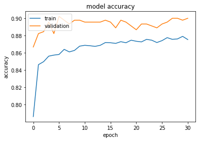
Loss and accuracy are rapidly stabilizing. The small value of the patience parameter used for early stopping caused a premature stop at epoch 31. The learning curves clearly show the presence of overfitting. Moreover, the statistics on the validation set are not stable.
This training is clearly not optimal!
5) Model evaluation
In the last step we can apply the model on the test set we split before.
Test loss: 0.2871
Test accuracy: 0.8700
The confusion matrix can also be obtained:
array([[306, 19], [ 46, 129]]) The performances of the model on the test set are comparable with the performances on the training and validation sets.
Conclusion
Obviously, the model presented here is far from being fully optimized! The first modifications to test, I can think of, are:
Train on more data
Modify the model architecture using other types of graph specialized layers
Optimize the hyperparameters
Change the classification objective used in this test, to a regression objective
But I hope that I could convince you that once you know the conversion pipe of molecules to graphs, the construction of a graph model is not so complicated 😉
All this work is the beginning for more tests and optimization cycles, and eventually an integration in one of our products. If you are interested to test this approach or another one from the deep learning world, come back to me, it will be a pleasure to collaborate with you!
Acknowledgments
I would like to warmly thank Daniele Grattarola for the discussions we had, his advice and the work he did on Spektral.
Thank you to all my colleagues for their comments on this post.
Code
The implementation of the code presented in this post is available here: https://github.com/Discngine/dng_dl_speknn
Useful links
References
Deep Learning for Deep Chemistry: Optimizing the Prediction of Chemical Patterns, Cova et Pais, Frontiers in Chemistry, 2019
A deep learning approach for the blind logP prediction in SAMPL6 challenge, Prasad et Brooks, J Comput Aided Mol Des, 2020
Deep learning for molecular design—a review of the state of the art, Elton et al., Molecular Systems Design & Engineering, 2019
ChemTS: An Efficient Python Library for de novo Molecular Generation, Yang et al., Comm. In Materials Informatics, 2017
Costless Performance Improvement in Machine Learning for Graph-Based Molecular Analysis, Na et al., JCIM, 2020